Math 132A

Bootstrapping

Variability of Statistics

  • In a statistical study, we collect a sample.
  • We then summarize the sample.
  • We can get some numerical summaries:
    • sample mean
    • sample proportion
    • sample standard deviation
    • …
  • Such sample summary is called a statistic.
  • Problem: each statistic will vary from sample to sample!
  • Question: how much can a statistic vary?

Random Variables and Distributions

  • A sample statistic obtained from a randomly collected sample is a number that is _determined through a random process.
  • Such numbers are called random variables.
  • Other examples:
    • A number rolled on a die.
    • Systolic blood pressure of a randomly selected patient.
    • Number of students in a randomly selected classroom in Science East.
    • …
  • We cannot predict what the number is going to be.
  • We can describe _what are all the possible values, and how likely is each of them to happen.
  • That is called a distribution of a random variable.

Sampling Distribution of a Statistic

  • We want to know how a particular sample statistic is distributed.
  • Such distribution is called a sampling distribution of the statistic.
  • To get that, we would have to repeatedly select a simple random sample from the population, and calculate the statistic, many many times.
  • Not practical!!!
    • Most of the time, even selecting one sample is already pretty hard.
  • What can we do instead?

Logic of Hypothesis Testing

  • Suppose we have some model, that we
    • either believe to be true,
    • or, want to check for validity.
  • (we called that the null model)
  • We can then simulate the sampling process, under the conditions described by the model.
  • That will tell us how would the sampling distribution look like if the model was true.
  • That is called a null distribution of the statistic.
  • We can then compare the observed value of the statistic with the null distribution to see how it fits.
  • We actually sample repeatedly from a fake population based on the null model.

Another Option: Bootstrapping

  • Sometimes we do not have a model to test, or the model is too hard to simulate.
  • We have one sample of size \(n\).
  • That is the only information we have about the population!
  • We can sample from a fake population based on the sample.
  • We say that we bootstrap the population from the sample.
  • The fake bootstrap population will look just like the sample, only much larger.
  • That can be done by sampling from the sample with replacement.
  • This is also called resampling.

Example (voters)

sample <- c("Yes", "Yes", "Yes", "Yes", "Yes", "Yes", "Yes", "Yes", "Yes",
            "Yes", "Yes", "No", "No", "No", "No", "No")
tally(sample)
X
 No Yes 
  5  11 

Resample:

resample(sample)
 [1] "Yes" "Yes" "Yes" "No"  "No"  "No"  "Yes" "Yes" "Yes" "No"  "Yes" "No" 
[13] "Yes" "Yes" "Yes" "Yes"

Resample again and tally:

tally(resample(sample))
X
 No Yes 
  5  11 

The Bootstrap Summaries

Resample many times:

do(10000) * tally(resample(sample)) -> bootstrap_data

This will produce the following data:

glimpse(bootstrap_data)
Rows: 10,000
Columns: 2
$ No  <int> 5, 9, 4, 4, 5, 8, 3, 4, 4, 6, 8, 5, 4, 6, 5, 7, 5, 3, 5, 4, 6, 4, …
$ Yes <int> 11, 7, 12, 12, 11, 8, 13, 12, 12, 10, 8, 11, 12, 10, 11, 9, 11, 13…

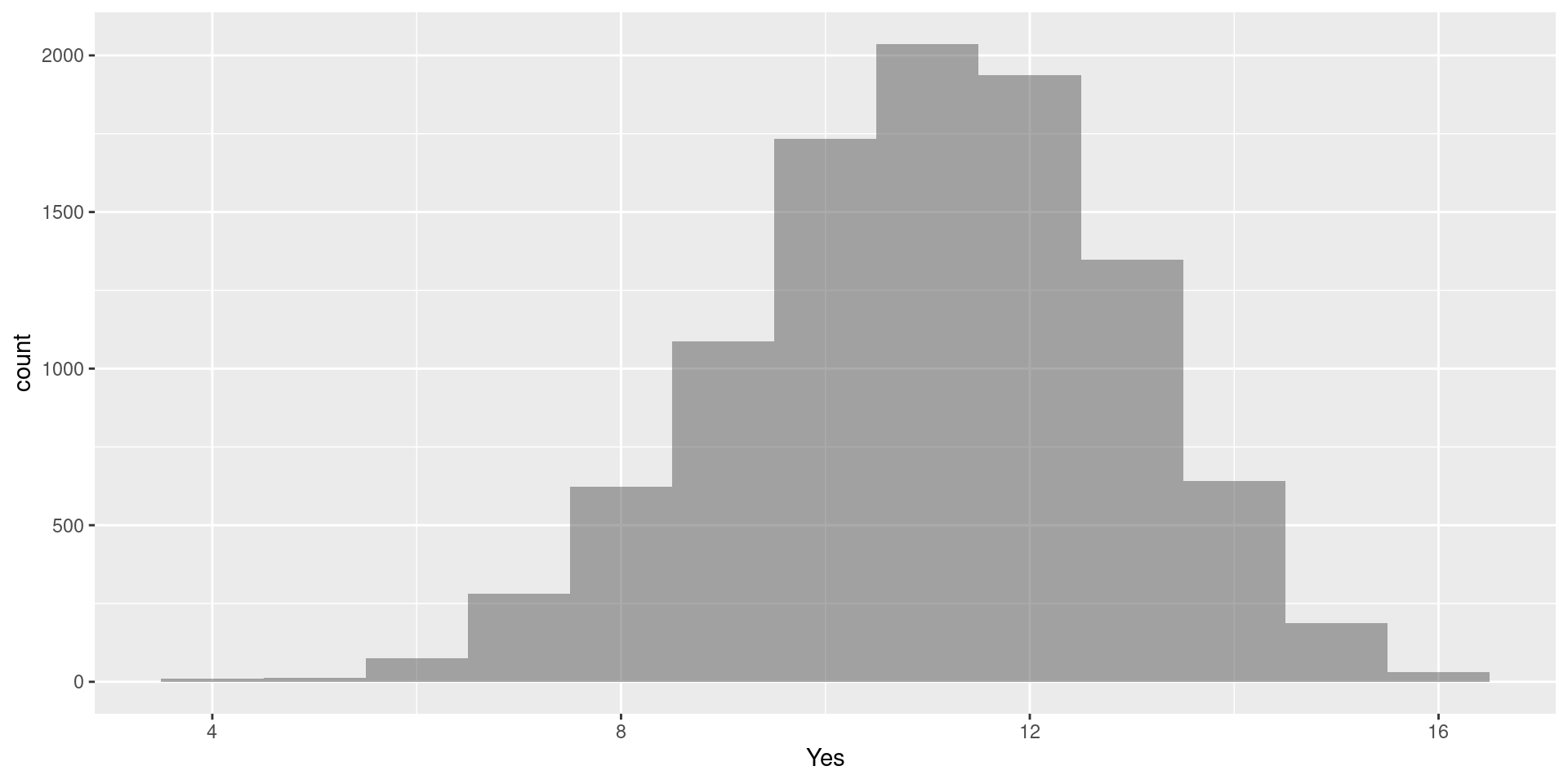
The Bootstrap Distribution:

gf_histogram(~Yes, data = bootstrap_data, binwidth = 1, boundary = 0.5)