Math 132A

Correlation and Linear Models

Two numerical variables

What is the association between them?
The first resource: scatterplot!
Options:
- No association
- linear association: correlation
- non-linear association
How “strong” is the correlation (if it exists)

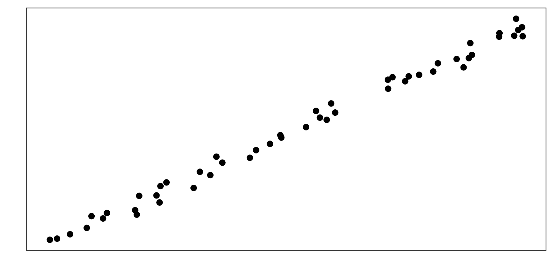
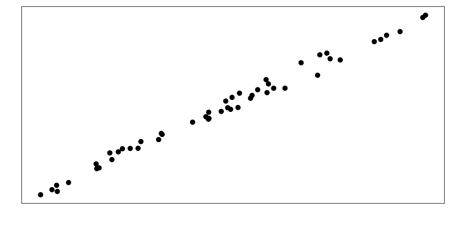
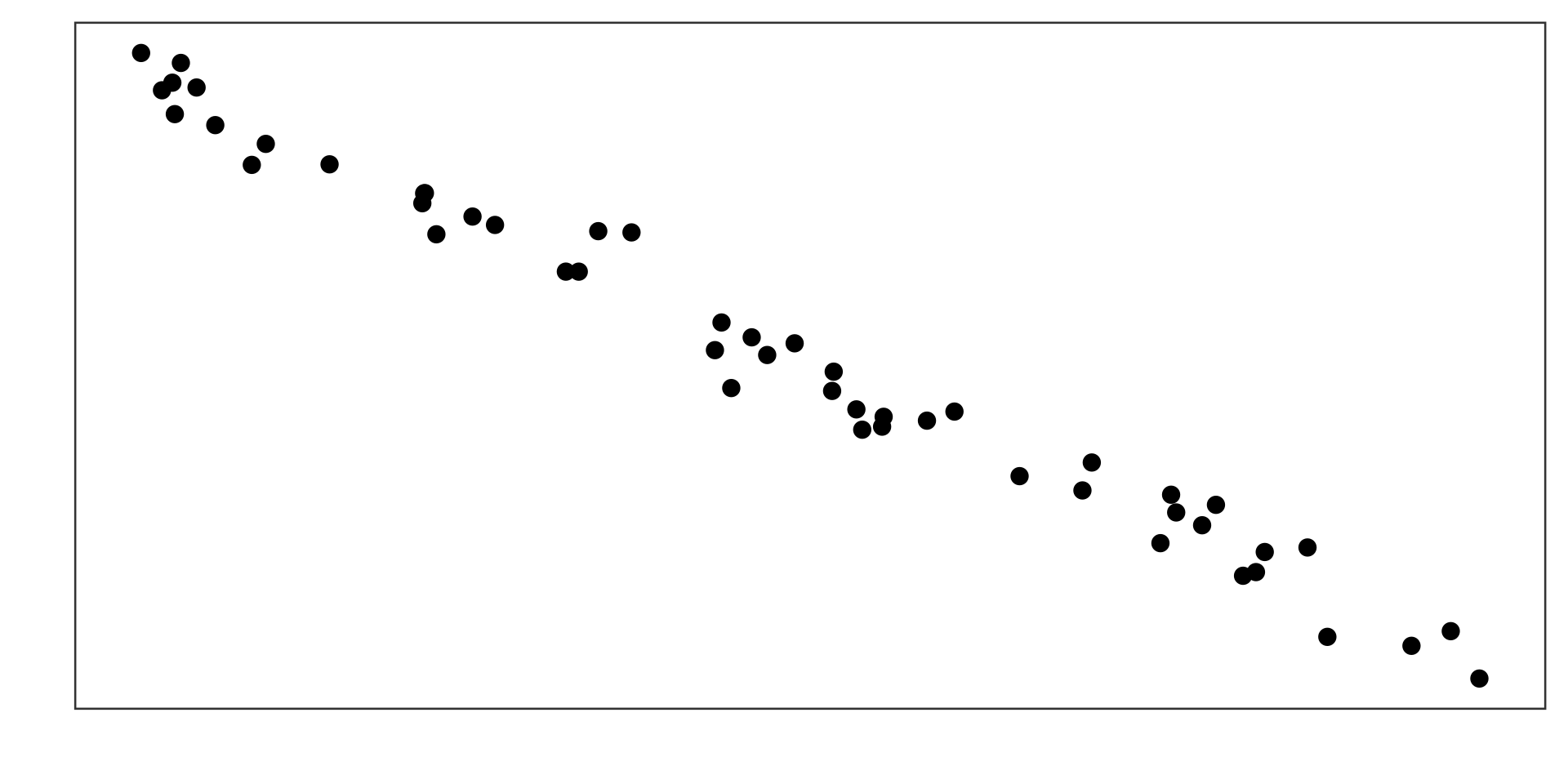
Strong positive correlation

Strong negative correlation

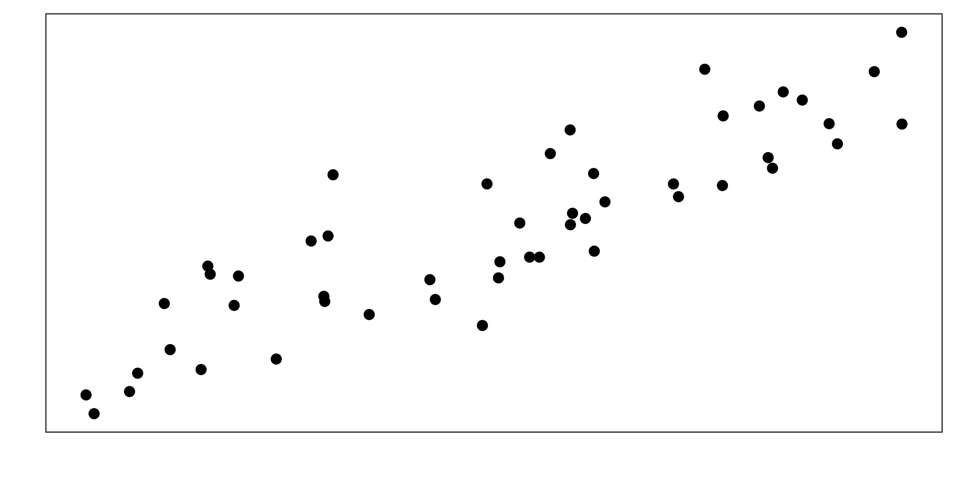
Weak positive correlation

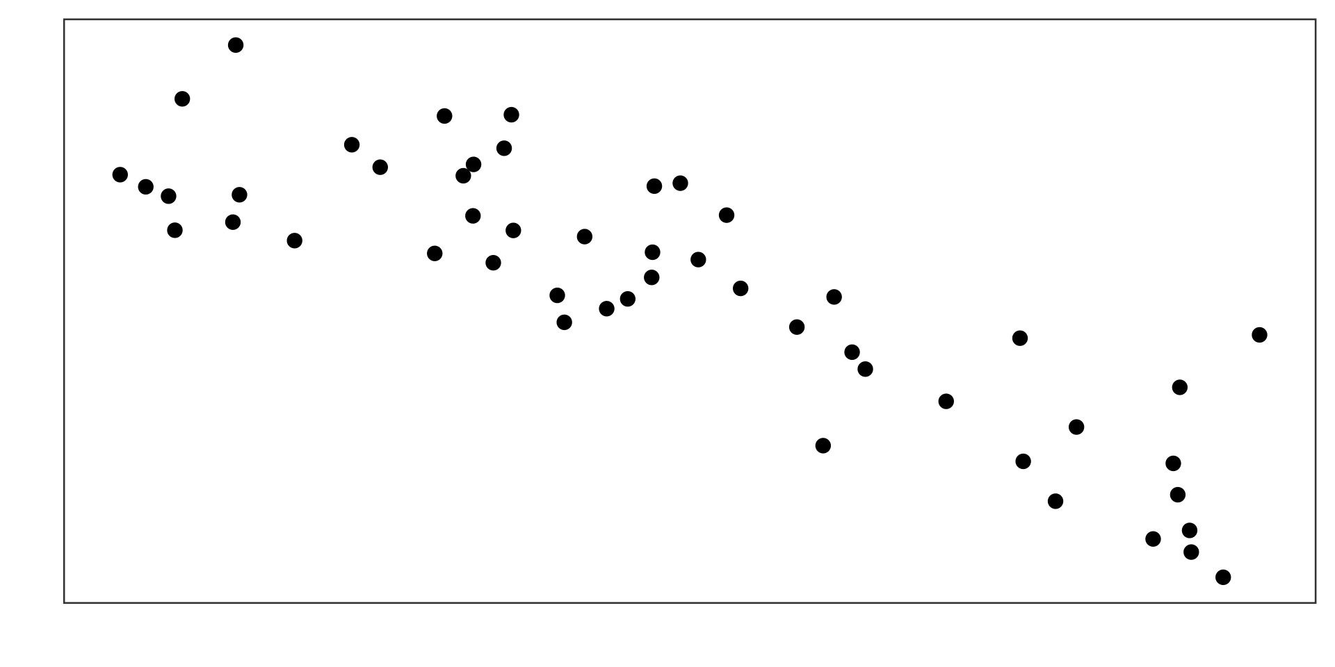
Weak negative correlation

Quadrants

General case

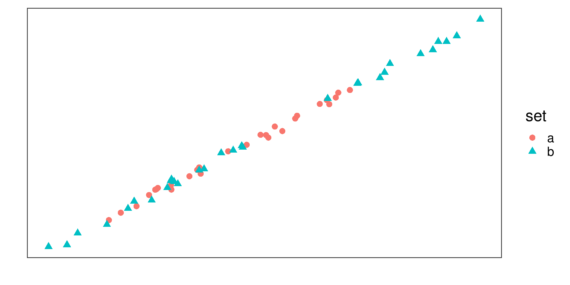
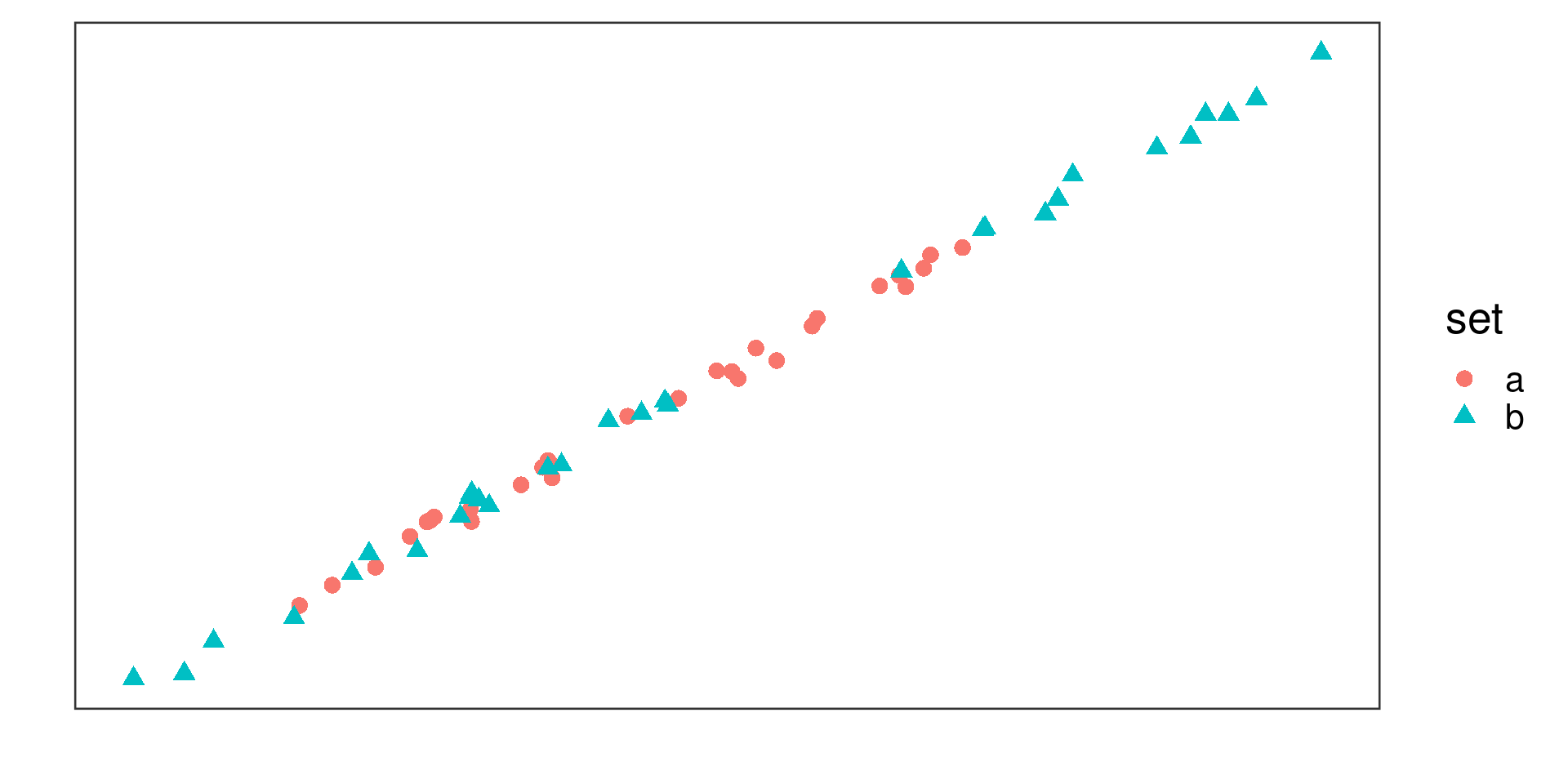
Not quite there yet

Mean of \((x- \overline{x})(y - \overline{y})\):

Set a: 1.478

Set b: 4.903

How to fix this problem?

Trying to use the mean of \((x - \overline{x})(y - \overline{y})\) to measure strength of correlation.
Two data sets with similar amount of “scatter” give us very different results: the data set with larger spread has larger deviations.
How do we measure spread?

Standard deviations:
- Set a: \(s_x = 1.4764001\) and \(s_y = 1.0384449\)
- Set b: \(s_x = 2.6967296\) and \(s_y = 1.8826342\)
An idea: divide each of the deviations by the corresponding standard deviation!

\[\text{Mean of } \frac{x - \overline{x}}{s_x} \frac{y - \overline{y}}{s_y}\]

Almost there

Mean of \(\frac{x- \overline{x}}{s_x}\frac{y - \overline{y}}{s_y}\):

Set a: 0.964

Set b: 0.966

Last (optional) adjustment

Mean of \(\frac{x- \overline{x}}{s_x}\frac{y - \overline{y}}{s_y}\):

\[\frac{1}{n}\sum\frac{x- \overline{x}}{s_x}\frac{y - \overline{y}}{s_y}\]
Small change to improve estimate properties:

\[\frac{1}{\color{red}{n-1}}\sum\frac{x- \overline{x}}{s_x}\frac{y - \overline{y}}{s_y}\]
Correlation coefficient \(r\)

Strong positive correlation

\(r = 0.995\)

Strong negative correlation

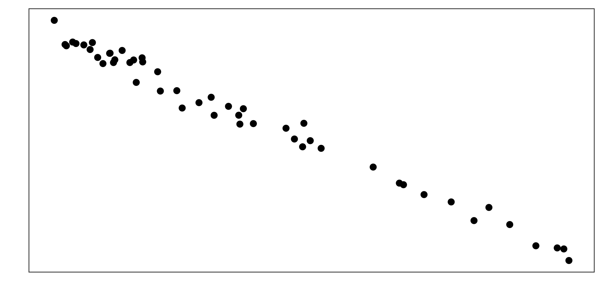
\(r = -0.993\)

Weak positive correlation

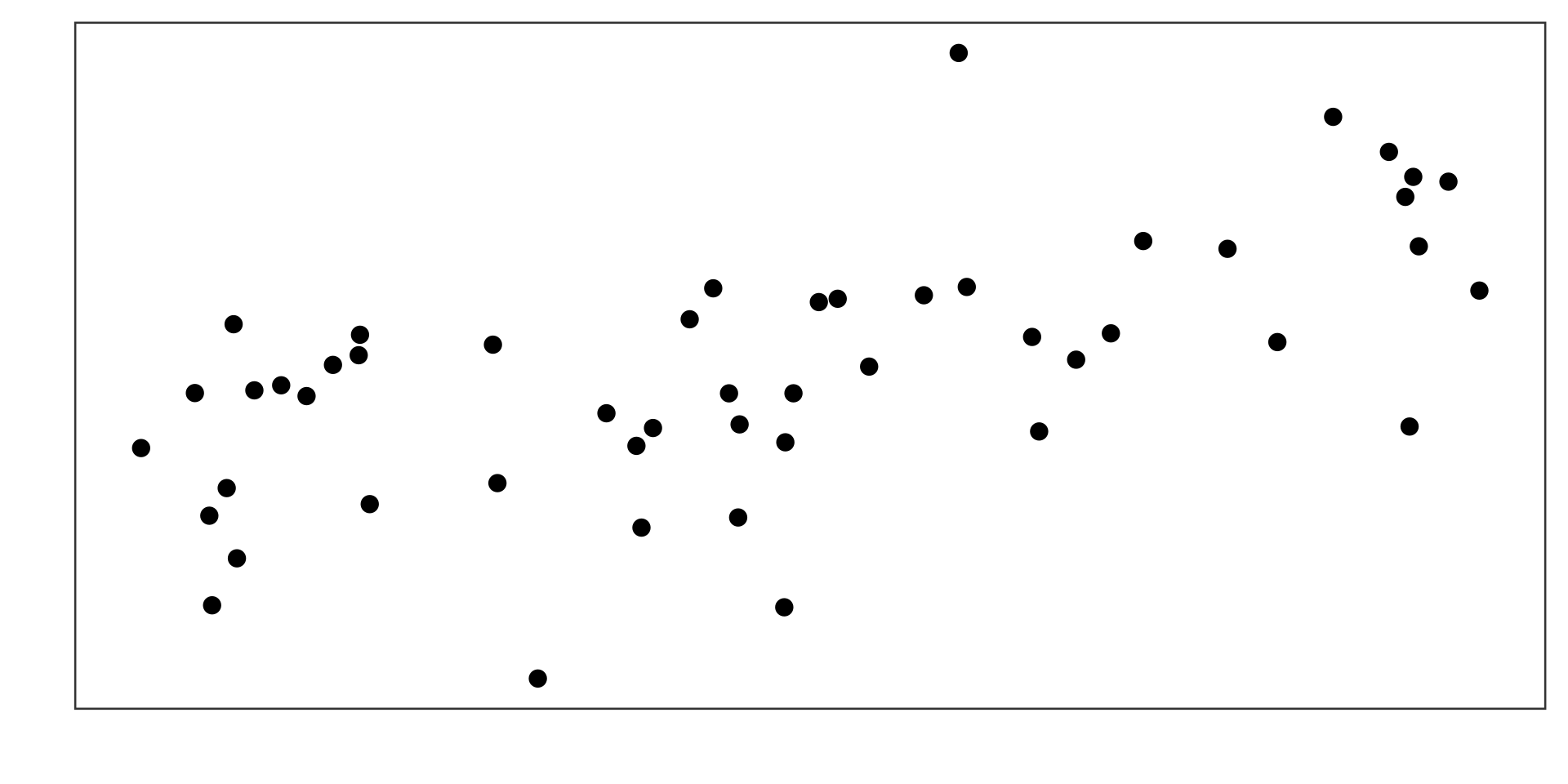
\(r = 0.611\)

Weak negative correlation

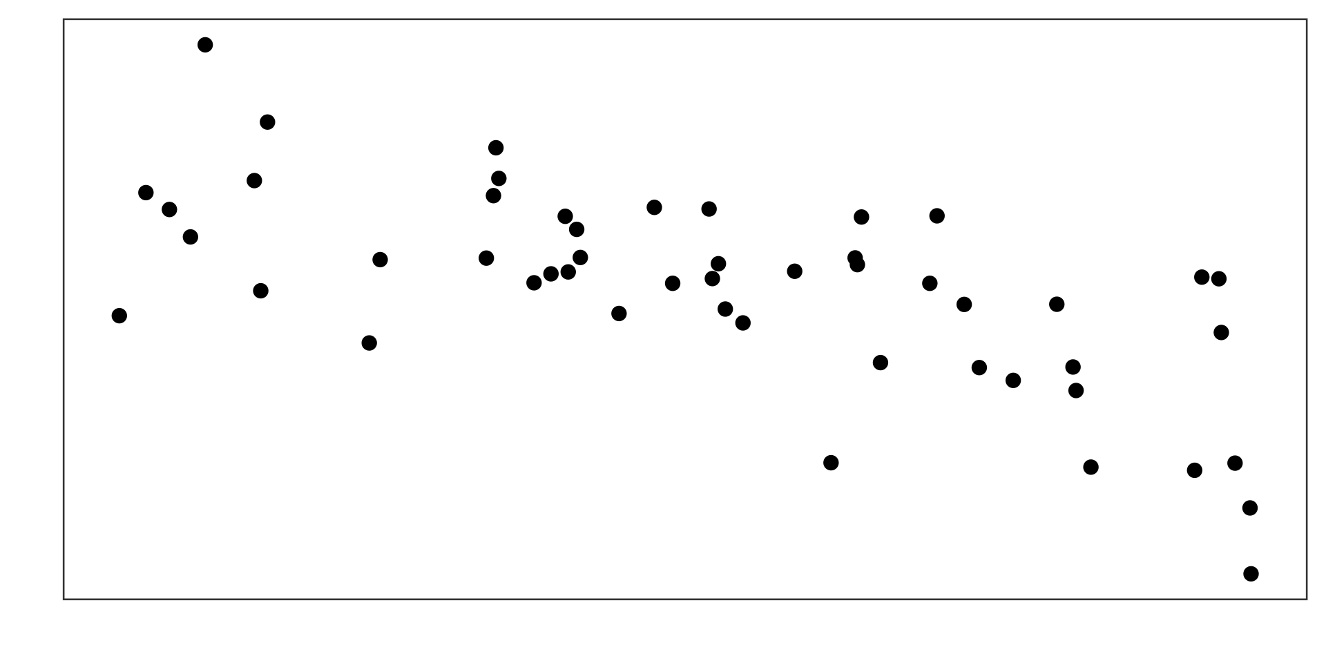
\(r = -0.672\)

Very weak positive correlation

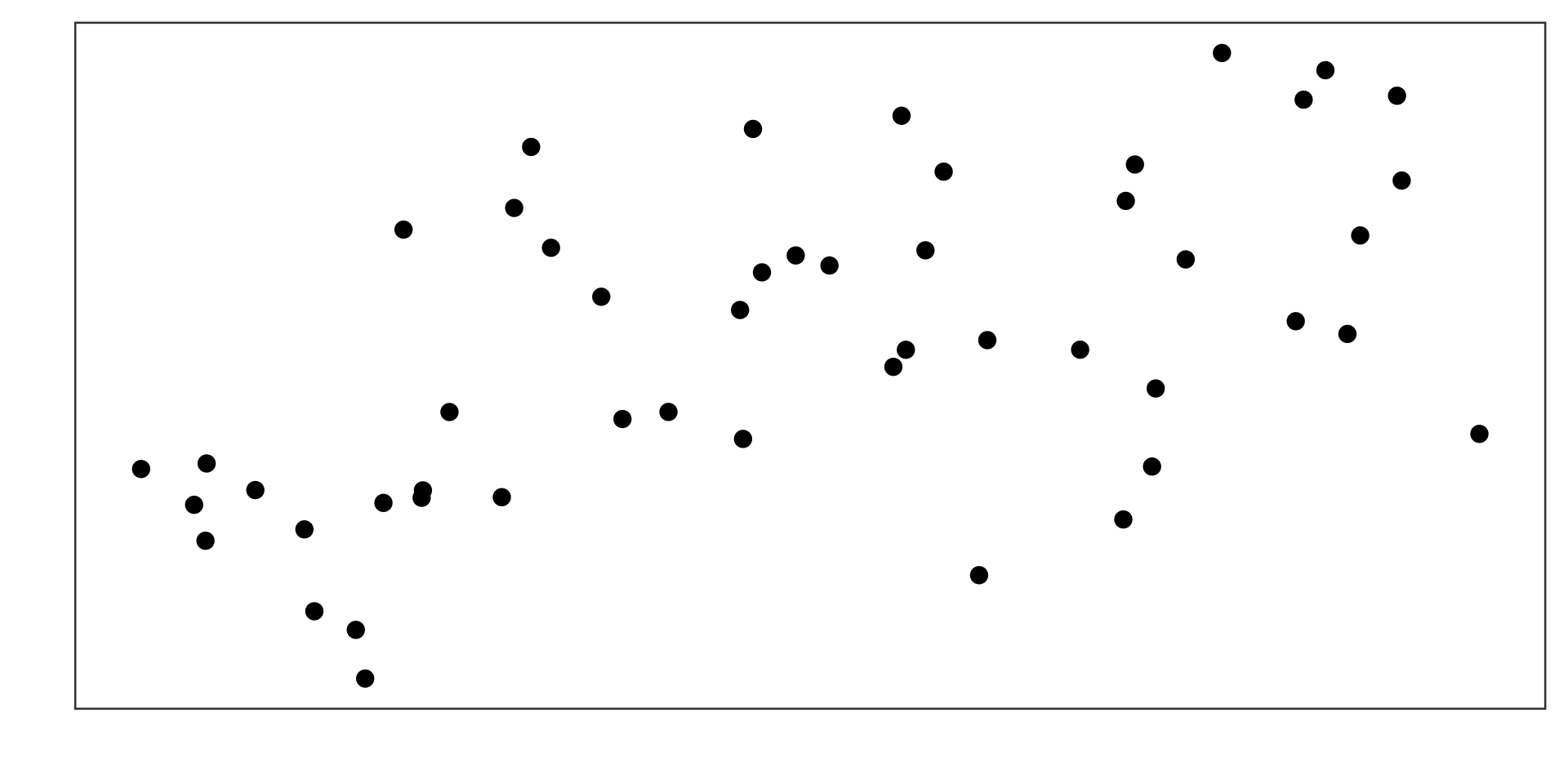
\(r = 0.561\)

Very weak negative correlation

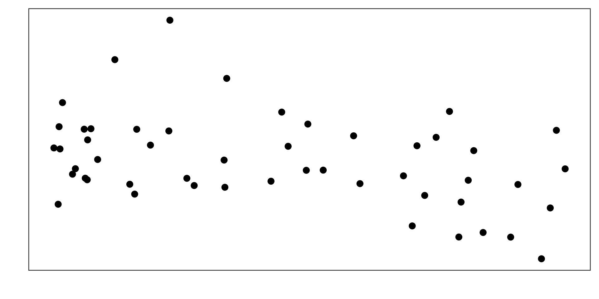
\(r = -0.391\)

No association

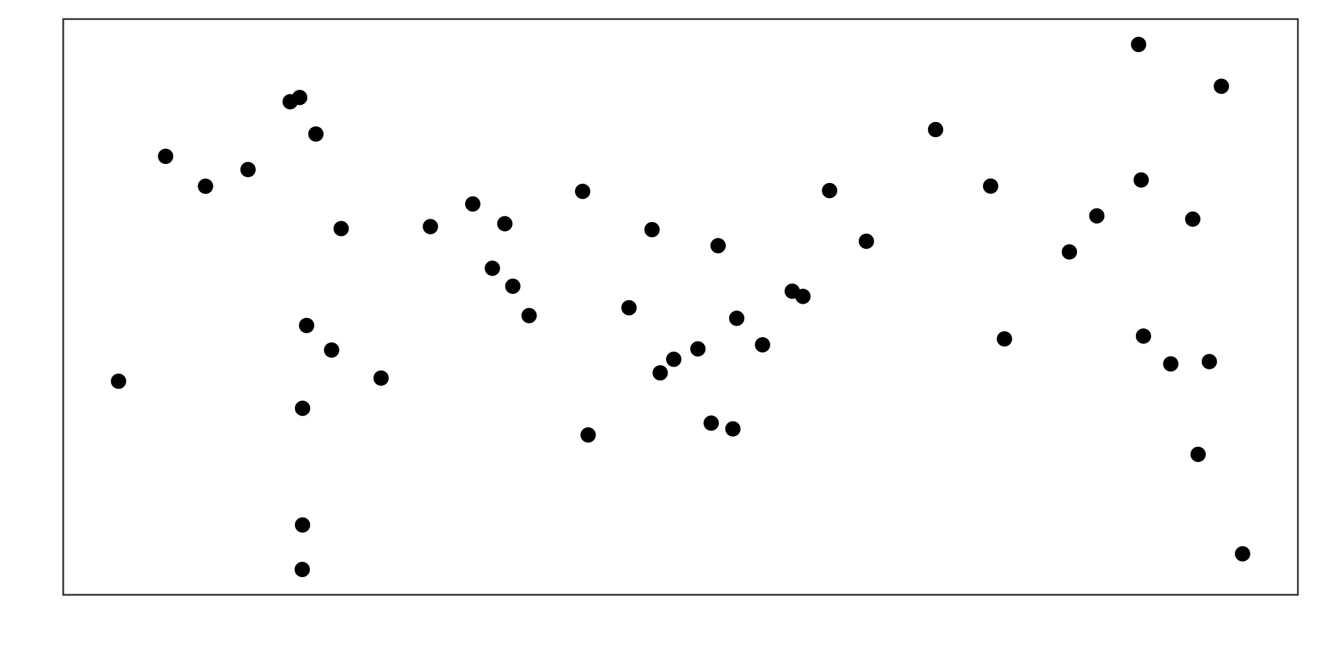
\(r = 0.003\)

Nonlinear association

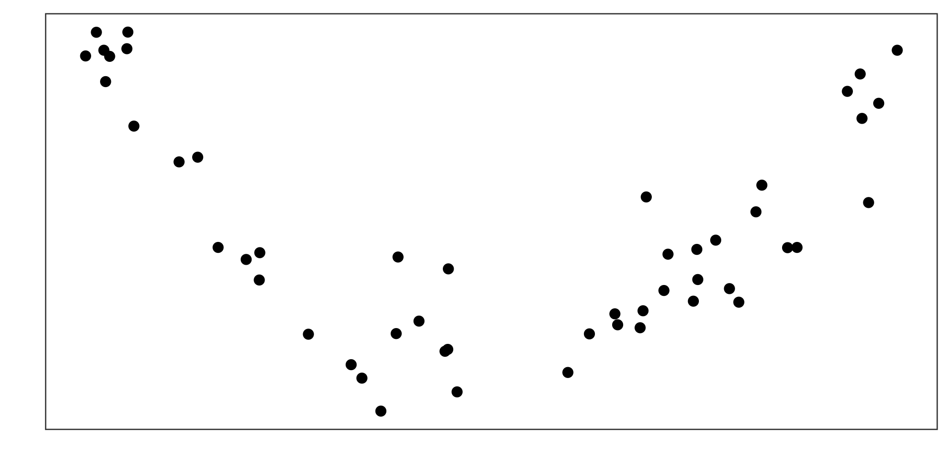
Correlation coefficient not useful!

Perfect positive correlation

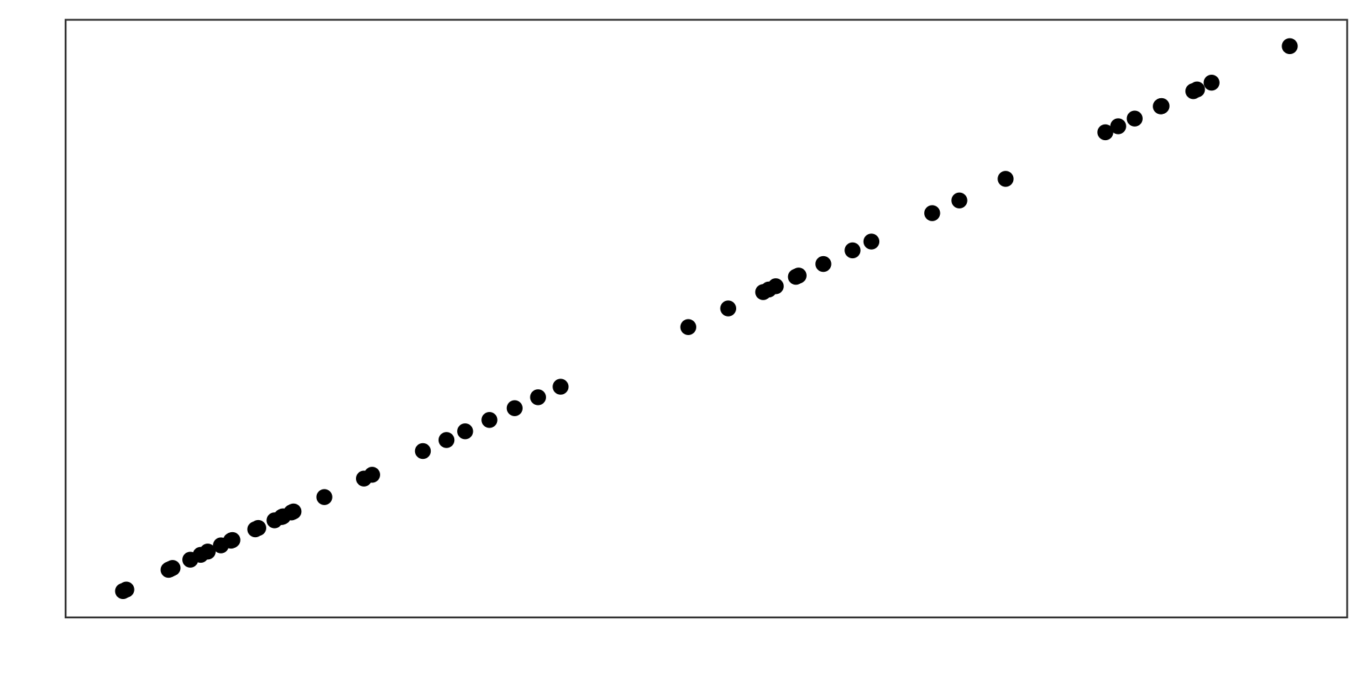
\(r = 1\)

Perfect negative correlation

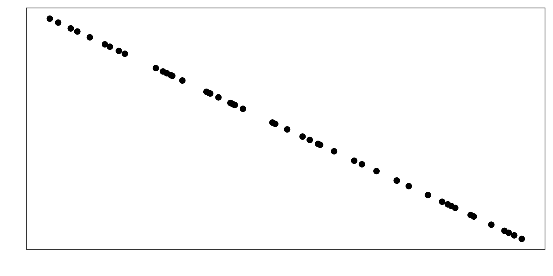
\(r = -1\)

Correlation Coefficient

\(\displaystyle\frac{1}{\color{red}{n-1}}\sum\frac{x- \overline{x}}{s_x}\frac{y - \overline{y}}{s_y}\)
Always between \(-1\) and \(1\).
Negative: negative correlation
Positive: positive correlation
\(\left\lvert r\right\rvert\) tells us the strength of the correlation.

Example

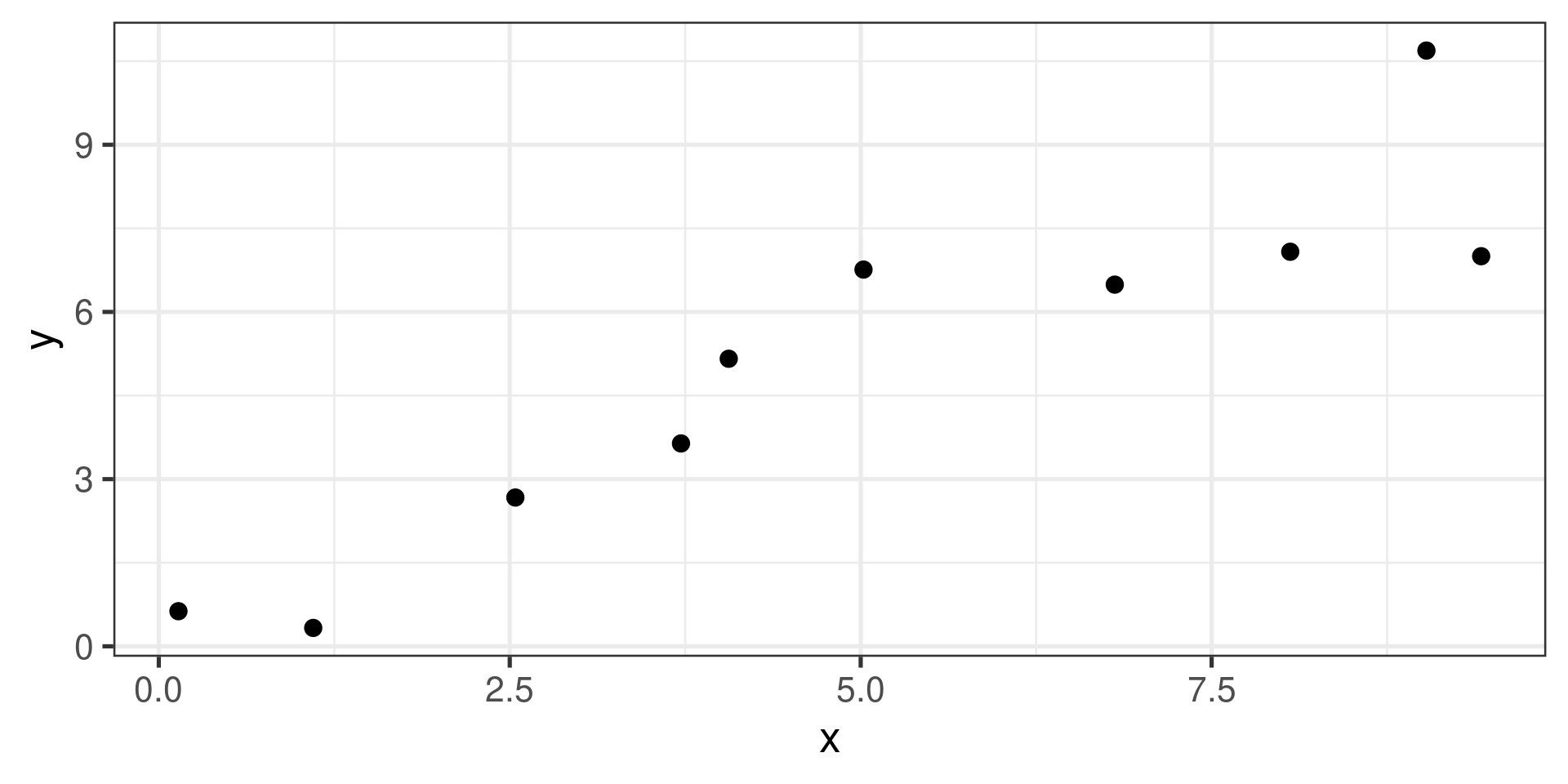
\(x\)	\(y\)	\(x - \overline{x}\)	\(y - \overline{y}\)	\((x - \overline{x})(y - \overline{y})\)
9.42	7	4.43	1.96	8.6828
6.81	6.49	1.82	1.45	2.639
9.03	10.69	4.04	5.64	22.7856
2.54	2.67	-2.45	-2.38	5.831
4.06	5.16	-0.93	0.12	-0.1116
0.14	0.63	-4.85	-4.42	21.437
1.1	0.33	-3.89	-4.72	18.3608
5.02	6.76	0.03	1.71	0.0513
3.72	3.64	-1.27	-1.4	1.778
8.06	7.08	3.07	2.04	6.2628
49.9	50.45			87.7167

Example (cont.)

Standard deviation of \(x\): 3.263
Standard deviation of \(y\): 3.235
Sum of \((x-\overline{x})(y-\overline{y})\): 87.7167
\(\displaystyle r = \frac{1}{n-1}\frac{\sum (x - \overline{x})\cdot(y - \overline{y})}{s_x\cdot s_y} = \frac{1}{9}\frac{87.7167}{3.263\cdot 3.235} = \color{red}{0.923}\)

Plot

Linear Models

So there is a correlation, and we can measure it’s strength.
What now?

We want to find a model for this association.

What is a Model?

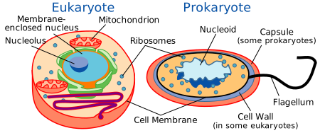
Image by Science Primer (National Center for Biotechnology Information).

What is a Model?

Geocentric model:

{
  const context = DOM.context2d(500, 600);
  while (true) {
    const t = Date.now() / 1000;
    const x = 500/2 + 200*(Math.cos(t));
    const y = 500/2 + 200*(Math.sin(t));
    const xp = x + 60*Math.cos(t/10);
    const yp = y + 60*Math.sin(t/10);
    const xs = 500/2 + 200*(Math.cos(t + Math.PI/2));
    const ys = 500/2 + 200*(Math.sin(t + Math.PI/2));
    context.clearRect(0, 0, 500, 600);
    context.beginPath();
    context.fillStyle="green";
    context.arc(500/2, 500/2, 20, 0, 2 * Math.PI);
    context.fill();
    context.beginPath();
    context.fillStyle="orange";
    context.arc(xs, ys, 10, 0, 2 * Math.PI);
    context.fill();
    context.beginPath();
    context.fillStyle="red";
    context.arc(xp, yp, 10, 0, 2 * Math.PI);
    context.fill();
    context.beginPath();
    context.moveTo(500/2,500/2);
    context.lineTo(xs,ys);
    context.stroke();
    context.beginPath();
    context.moveTo(500/2,500/2);
    context.lineTo(x,y);
    context.lineTo(xp,yp);
    context.stroke();
    yield context.canvas;
  }
}

Heliocentric model:

{
  const context = DOM.context2d(500, 600);
  while (true) {
    const t = Date.now() / 1000;
    const xe = 500/2 + 100*(Math.cos(t/10));
    const ye = 500/2 + 200*(Math.sin(t/10));
    const xp = 500/2 + 130*(Math.cos(t/18 + Math.PI/3));
    const yp = 500/2 + 250*(Math.sin(t/18 + Math.PI/3));
    context.clearRect(0, 0, 500, 600);
    context.beginPath();
    context.fillStyle="yellow";
    context.arc(500/2, 1500/4, 20, 0, 2 * Math.PI);
    context.fill();
    context.beginPath();
    context.fillStyle="green";
    context.arc(xe, ye, 10, 0, 2 * Math.PI);
    context.fill();
    context.beginPath();
    context.fillStyle="red";
    context.arc(xp, yp, 10, 0, 2 * Math.PI);
    context.fill();
    yield context.canvas;
  }
}

What is a Model?

What are models good for?

To understand how the world works

To predict, calculate or plan practical solutions

Why?

All models are wrong …

but some are useful.

George Box

Linear Models

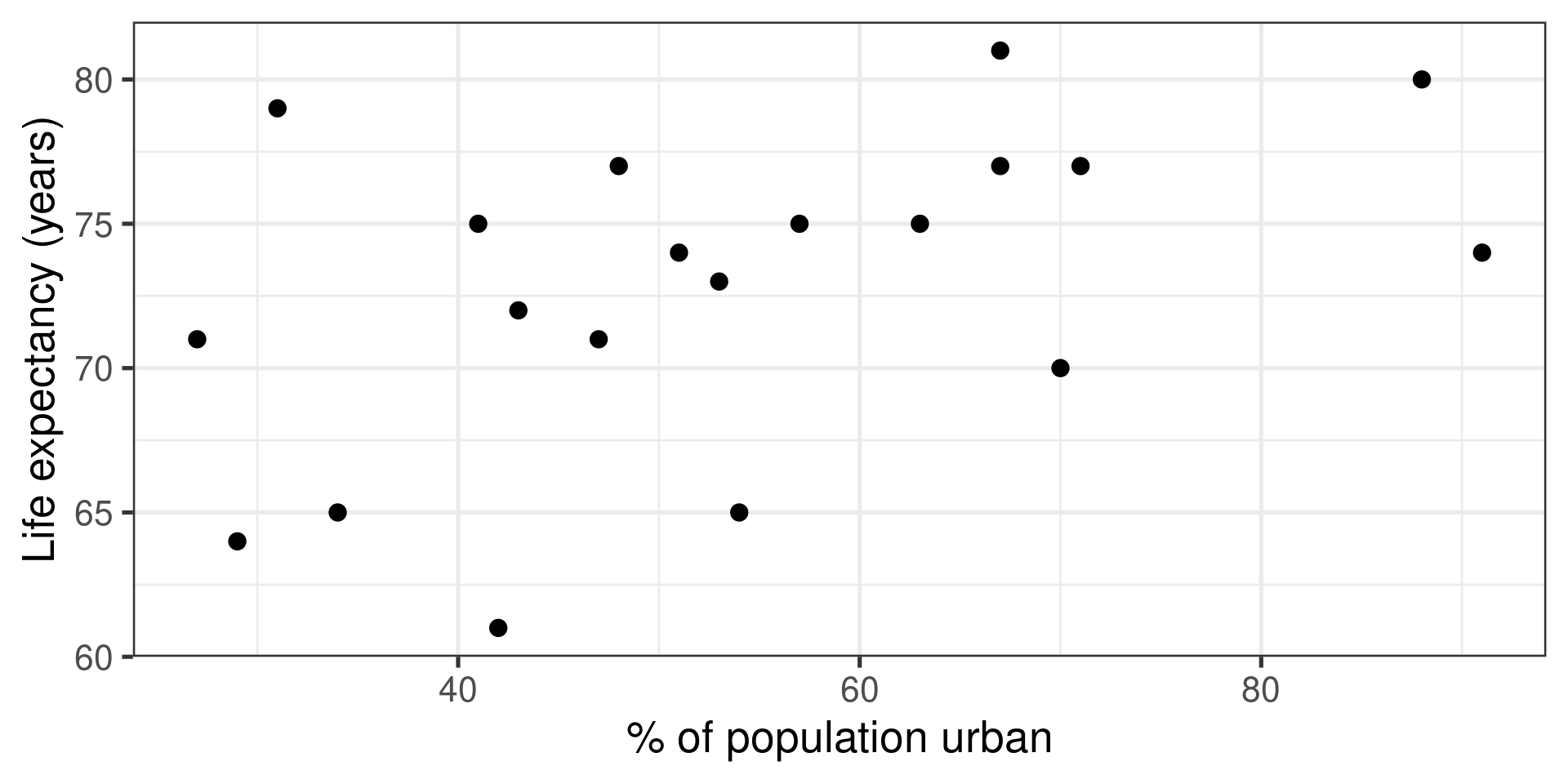
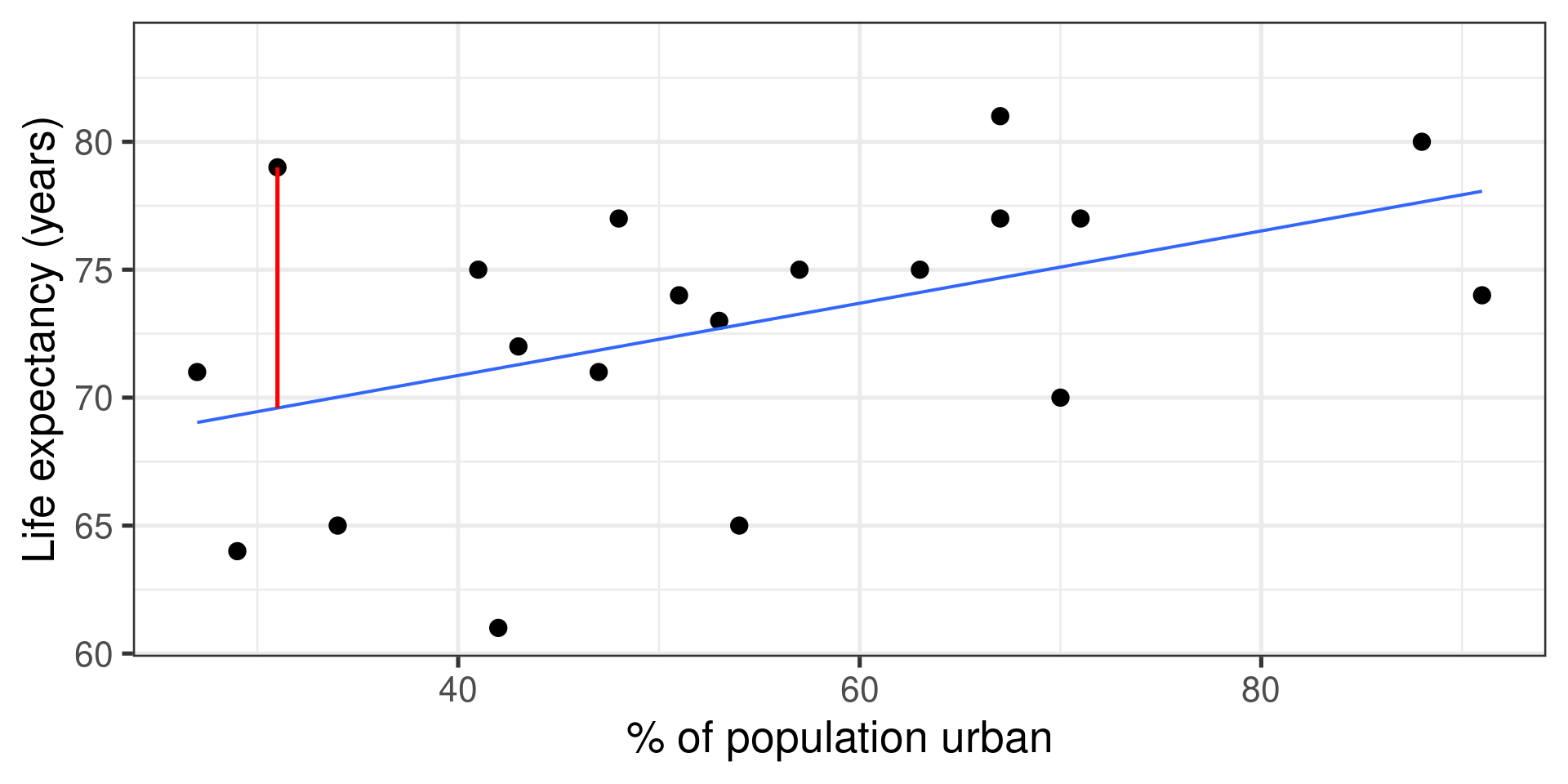
What is the relationship between urban population and life expectancy?
Can we predict life expectancy of a country if we know what percent of population is urban?
- What is the formula?
- How good are the predictions?
If a country increases its urban population by 1%, how is the life expectancy going to change?

Linear Models

A linear model provides answers to these questions.
It gives us a formula for calculating predicted values of life expectancy from percent of population urban.
- It does not have to be a linear function of the percent of urban population!
- It does have to be a linear function of the coefficients!
- \(\widehat{y} = b_0 + b_1x + b_2x^2\) is a linear model.
- \(\widehat{y} = b_0 + b_1x + \sqrt{b_2 + x^2}\) is not!

Linear Models

There seems to be a linear association between life expectancy and percent of population urban.
This linear model should take a form of a linear function.
Notation: \(\widehat{\text{life expectancy}}\): the predicted value of the life expectancy variable, according to the model.
Notation: \(b_0\): the intercept of the linear function.
Notation: \(b_1\): the slope of the linear function.

Linear Models

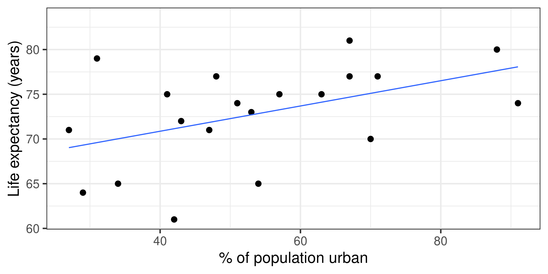
\[\widehat{\text{life expectancy}} = b_0 + b_1 \times \text{percent population urban}\]

For example:

\[\widehat{\text{life expectancy}} = 65.22 + 0.14 \times \text{percent population urban}\]

Linear Models

Predicted value: \(\widehat{\text{life expectancy}}\)
Actual (observed) value: \({\text{life expectancy}}\)
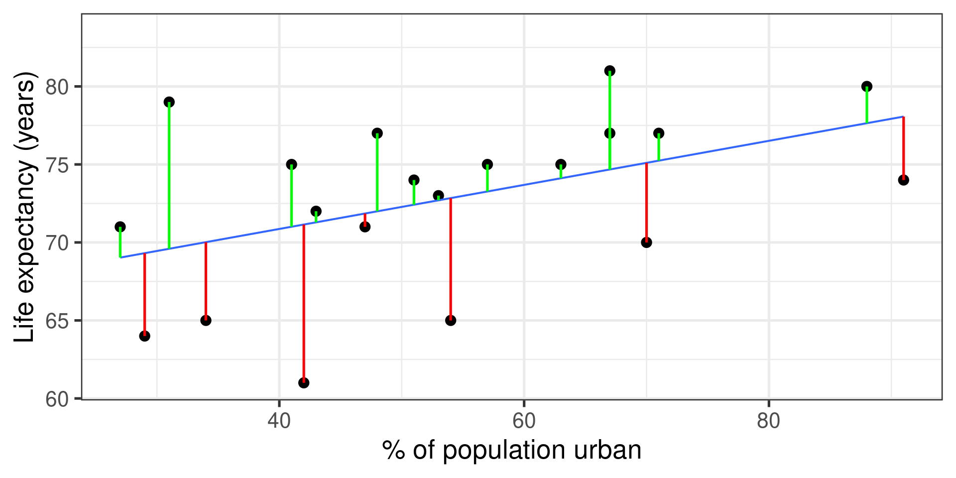
Prediction error: \(e = {\text{life expectancy}} - \widehat{\text{life expectancy}}\)

Linear Models

Example:

Country: Barbados
percent urban population: 31
actual life expectancy: 79

Predicted life expectancy: \(65.22 + 0.14 \times 31 = 69.59\)

Prediction error: \(79 - 69.59 = 9.41\)

Linear Models

Prediction Errors (Residuals)

Summary

Model of a linear association between \(x\) and \(y\):

Actual (observed) value: \(y\)
Predicted value: \(\widehat{y} = b_0 + b_1 x\)
Prediction error (residual): \(e = y - \widehat{y}\)
Observed value again: \(y = \widehat{y} + e = b_0 + b_1 x + e\)