Math 132A

Hypothesis Testing Examples

Another Study Example (modified)

A group of residents of a county is considering submitting a question on certain matter for a local referendum in the next election cycle. Submitting a question for a referendum requires a fair amount of work, as well as large financial commitment, so before they do all that, they want to find out whether there is sufficient support for the matter in the county.

They select a simple random sample of 36 eligible voters in the county and ask them if they would support the measure.

Out of the 36 voters, 23 responded that they would support the matter, while the remaining 13 would not.

Should the group go ahead with the submission?

Null Model and Hypotheses

Null model:
- Exactly 50% of the voters in the county support the measure.
- (That is the highest level of support that would not be sufficient for passing the measure)
Null hypothesis: \(H_0: p = 0.5\).
Alternative hypothesis: \(H_A: p > 0.5\).
Rejecting the null model means there is a sufficient support for the measure.

Simulation

Flip 36 coins with probability of head 0.5.
Count the number of heads.
Repeat many times
```
do(10000) * rflip(36) -> flips
```

Ask how often we got 23 or more heads

tally(~(heads >= 23), data = flips, format = "proportion")

(heads >= 23)
 TRUE FALSE 
0.064 0.936

If the null model is correct, there is 6.4 percent chance that a simple random sample of size 36 will have 23 or more voters supporting the measure.

Simulated Null Distribution

gf_histogram(~heads, data = flips, binwidth = 1, boundary = -0.5, fill = ~(heads >= 23))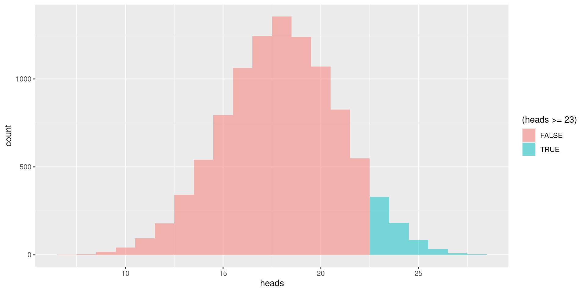

Central Limit Theorem

Success-failure condition:
- \(np = 36\cdot 0.5 = 18 \ge 10\) and \(nq = 36\cdot 0.5 = 18 \ge 10\).
Standard error: \[SE = \sqrt{36\cdot 0.5\cdot 0.5} = 3.\]
Null distribution: \[\overline{X} \sim N(18, 3)\]
Assuming the null model is correct, the probability that there will be 23 or more voters supporting the measure in a simple random sample of size 36 is
```
1 - pnorm(22.5, mean = 18, sd = 3)
```
```
[1] 0.0668072
```

Theoretical Null Distribution

gf_dist("norm", mean = 18, sd = 3, fill = ~(x >= 22.5), geom = "area")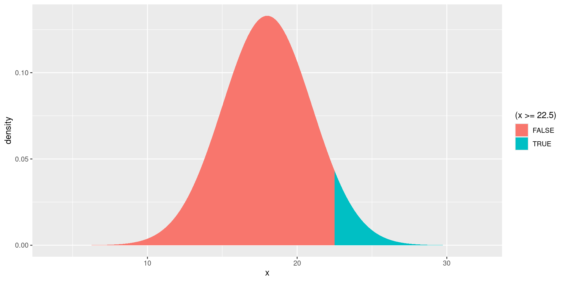

Comparison of Both Distributions

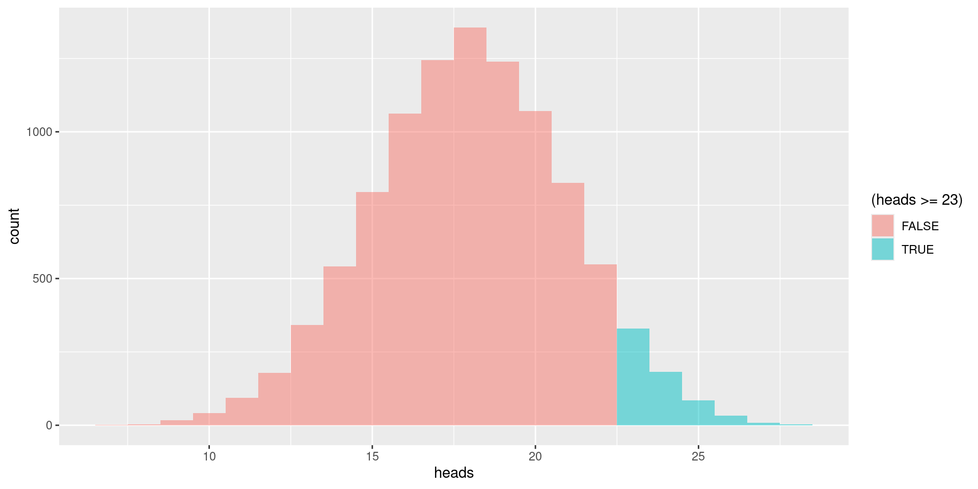
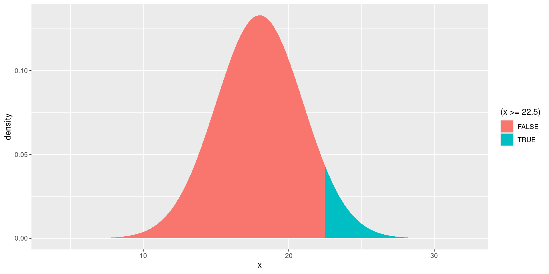
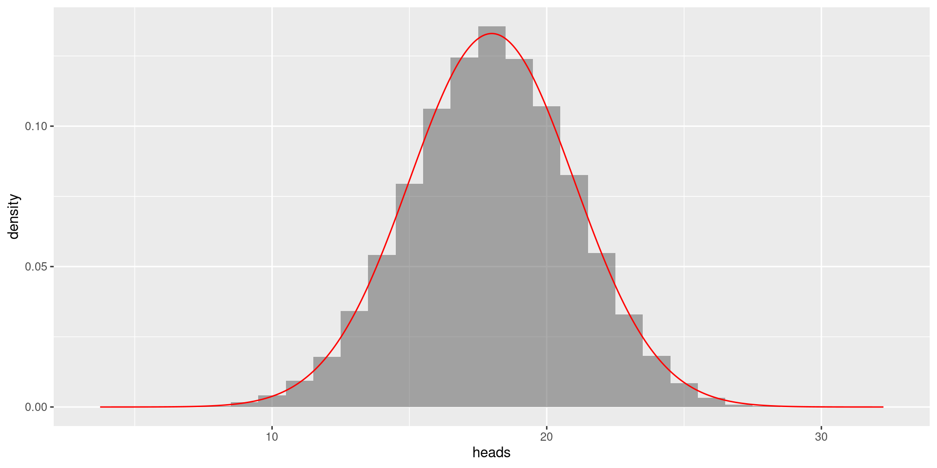
P-Value

Question: How well does the null model explain the observed results?

Another way to put this: Assuming the null model is true, what is the probability of getting a sample like the one we observed, or even more extreme.

This probability is called the p-value of the sample.

In our example:

p-value obtained by simulation:

prop(~(heads >= 23), data = flips)

prop_TRUE 
    0.064

theoretical p-value from the CLT:

1 - pnorm(22.5, mean = 18, sd = 3)

[1] 0.0668072

Conclusion?

If the p-value is large, the null model is a plausible explanation for the observed data.
If the p-value is small, the null model does not explain the observed data very well.

What does it mean “small”?

Smaller than some previously chosen significance level \(\alpha\).

Commonly chosen values for \(\alpha\): 5%, 10%, 2%, 1%, …

Assuming we chose \(\alpha = .05\), our p-value is larger than \(\alpha\).

We do not reject the null model!

At 5% significance level, it is plausible that the level of support for the measure in the county is exactly 50%.

Example for Means

A company producing bottled water claims that the mean volume of water in their bottles as at least 17 oz. A quality control engineer investigating this claim selected a random sample of 100 bottles produced by this company. She discovered that the mean water volume in this sample was 16.84 oz, with standard deviation of .5 oz.

At 5% significance level, is the company’s claim consistent with her sample?

Null hypothesis: \(H_0: \mu = 17\).

Alternative hypothesis: \(H_A: \mu < 17\).

\(n = 100\)
\(\overline{x} = 16.84\)
\(s = 0.5\)

Standard Error: \[SE = \frac{s}{\sqrt{n}} = \frac{0.5}{\sqrt{100}} = 0.05.\]

T-statistic

Null hypothesis: \(H_0: \mu = 17\).

Alternative hypothesis: \(H_A: \mu < 17\).

\(n = 100\)
\(\overline{x} = 16.84\)
\(s = 0.5\)

Standard Error: \[SE = \frac{s}{\sqrt{n}} = \frac{0.5}{\sqrt{100}} = 0.05.\]

\[t = \frac{\overline{x} - \mu}{SE} = \frac{16.84 - 17}{.05} = \frac{-.16}{.05} = -3.2\]

\[T \sim T(99)\]

We need to know the probability that \(T \le -3.2\).

With 99 degrees of freedom, the \(T(99)\) and \(N(0,1)\) are very close to each other.

Using Standard Normal Distribution

gf_dist("norm", mean = 0, sd = 1) |> gf_vline(xintercept = -3.2, color="red")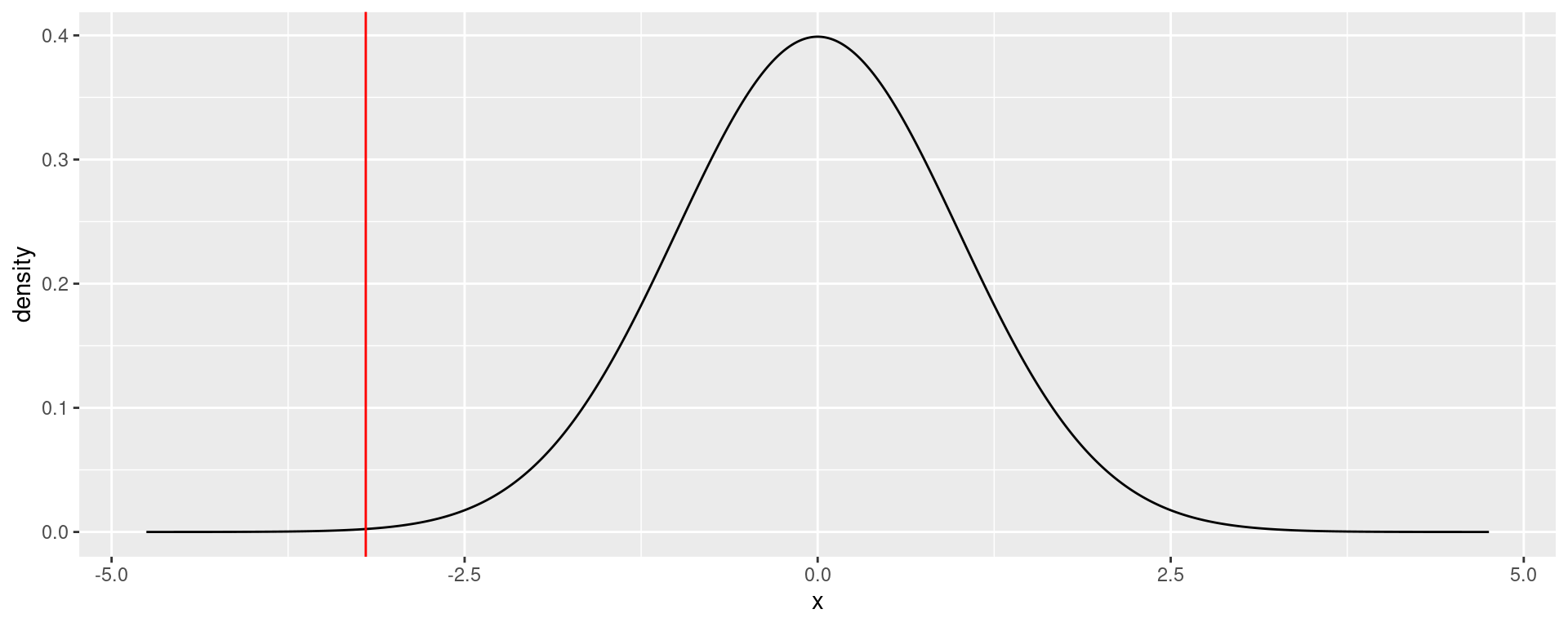

pnorm(-3.2)

[1] 0.0006871379

Using T Distribution

gf_dist("t", df = 99) |> gf_vline(xintercept = -3.2, color="red")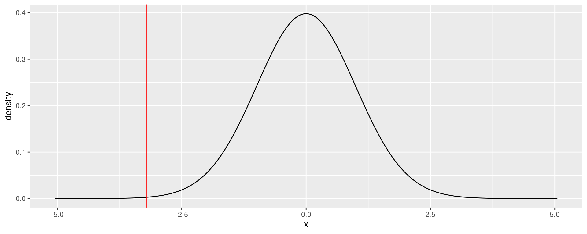

pt(-3.2, df = 99)

[1] 0.0009235327

Conclusion

P-value:
- 0.0006871 using standard normal distribution
- 0.0009235 using \(T(99)\) distribution
Significance level \(\alpha = 0.05\)
P-value is less than \(\alpha\), so the null model does not explain the data well.
At 5% significance level, we reject the null hypothesis that the mean volume of water in the bottles is 17 oz.

Procedure for Hypotheses Testing

Choose your significance level \(\alpha\) (e.g. 5%).
Choose whether you want two-sided (default) or one-sided test.
Formulate your \(H_0\) (must have equality) and \(H_A\).
Choose sample size \(n\).
Collect your data.
Verify assumptions!!!!
- Is your sample large enough?
From the data, calculate the point estimate and anything else you need.
Calculate the standard error \(SE\).
Calculate the test statistic.
Determine the \(p\)-value.
Compare the \(p\)-value with the significance level \(\alpha\).
Write down the conclusion.

Procedure for Hypotheses Testing

Choose your significance level \(\alpha\) (e.g. 5%).
Choose whether you want two-sided (default) or one-sided test.
Formulate your \(H_0\) (must have equality) and \(H_A\).
Choose sample size \(n\).
Collect your data.
Simulate sampling from the null model.
Determine the \(p\)-value.
Compare the \(p\)-value with the significance level \(\alpha\).
Write down the conclusion.