Math 132A

Line of Best Fit

Summary

Model of a linear association between \(x\) and \(y\):

  • Actual (observed) value: \(y\)

  • Predicted value: \(\widehat{y} = {\color{#44ee44}b_0} + {\color{#44ee44}b_1} x\)

  • Prediction error (residual): \(e = y - \widehat{y}\)

  • Observed value again: \(y = \widehat{y} + e = {\color{#44ee44}b_0} + {\color{#44ee44}b_1} x + e\)

How do we find \(b_0\) and \(b_1\)?

Minimizing residuals

We want the prediction errors or residuals to be as small as possible.

There is one residual for each observation.

Some are positive while others are negative.

Try to make the sum of squares of residuals as small as possible.

Sum of Squares

Formulas for the Coefficients

What we need:

  • The correlation coefficient \(r\)
  • The mean of the \(x\) variable: \(\overline{x}\)
  • The mean of the \(y\) variable: \(\overline{y}\)
  • The standard deviation of the \(x\) variable: \(s_x\)
  • The standard deviation of the \(y\) variable: \(s_y\)

\[b_1 = \frac{s_y}{s_x}\cdot r\]

\[b_0 = \overline{y} - b_1\cdot\overline{x}\]

\[\widehat{y} - \overline{y} = b_1\cdot \left(x - \overline{x}\right)\]

Our Example

What we need:

  • \(r = 0.47\)
  • \(\overline{x} = 53.7\)
  • \(\overline{y} = 72.8\)
  • \(s_{x} = 18.22\)
  • \(s_{y} = 5.53\)

\[ \begin{aligned} b_1 &= \frac{s_y}{s_x}\cdot r\\[1.3ex] &= \frac{5.53}{18.22}\cdot 0.47\\[1.3ex] &= 0.14 \end{aligned} \]

\[ \begin{aligned} b_0 &= \overline{y} - b_1\cdot\overline{x}\\[1.3ex] &= 72.8 - 0.14\cdot 53.7\\[1.3ex] &= 65.28 \end{aligned} \]

\[\widehat{y} = 65.28 + 0.14 x\]

Using R

glimpse(sowc_sample)
Rows: 20
Columns: 3
$ countries_and_areas  <chr> "Guatemala", "Trinidad and Tobago", "Philippines"…
$ percent_urban_2018   <int> 51, 53, 47, 27, 67, 31, 43, 91, 48, 41, 71, 63, 5…
$ life_expectancy_2018 <int> 74, 73, 71, 71, 81, 79, 72, 74, 77, 75, 77, 75, 7…
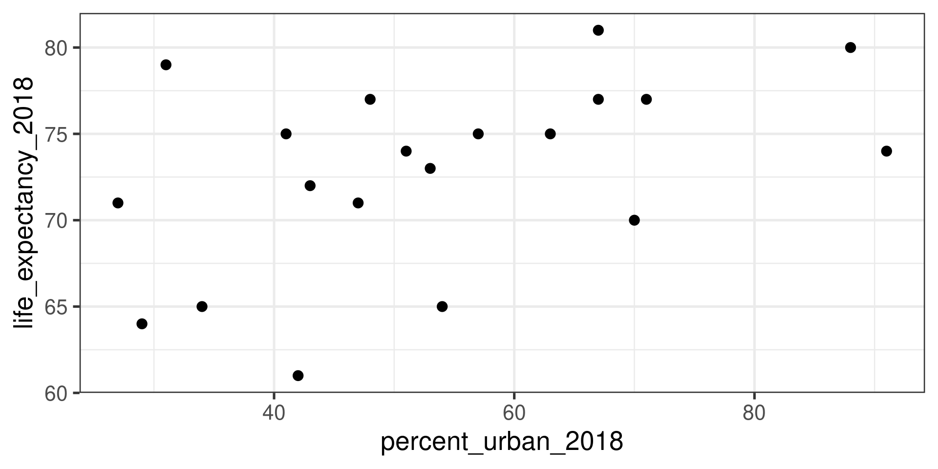
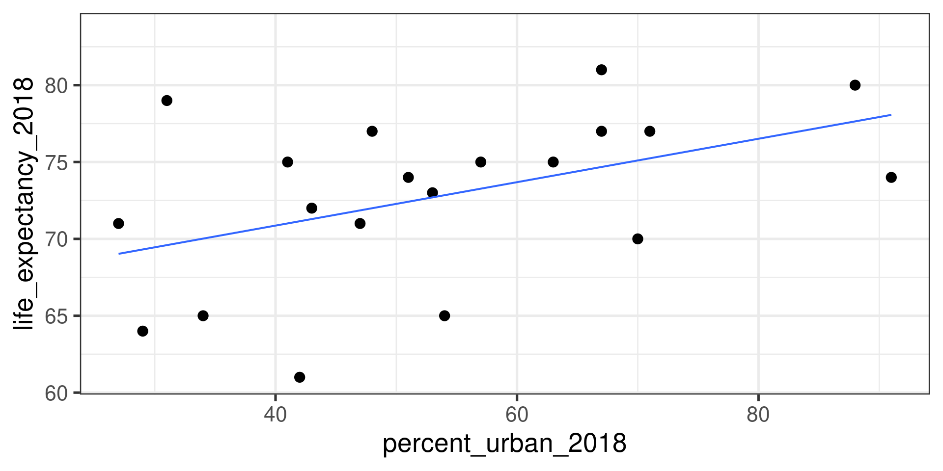
Question: How do we predict life expectancy from percent urban population?

Scatterplot

gf_point(life_expectancy_2018 ~ percent_urban_2018, data = sowc_sample)

Correlation and Linear Model

cor(life_expectancy_2018 ~ percent_urban_2018, data = sowc_sample)
[1] 0.4652268


model <- lm(life_expectancy_2018 ~ percent_urban_2018, data = sowc_sample)

model

Call:
lm(formula = life_expectancy_2018 ~ percent_urban_2018, data = sowc_sample)

Coefficients:
       (Intercept)  percent_urban_2018  
           65.2169              0.1412  

Summary of the Model

summary(model)

Call:
lm(formula = life_expectancy_2018 ~ percent_urban_2018, data = sowc_sample)

Residuals:
    Min      1Q  Median      3Q     Max 
-10.148  -4.305   1.234   2.330   9.405 

Coefficients:
                   Estimate Std. Error t value Pr(>|t|)    
(Intercept)        65.21686    3.58200   18.21 4.84e-13 ***
percent_urban_2018  0.14121    0.06333    2.23   0.0387 *  
---
Signif. codes:  0 '***' 0.001 '**' 0.01 '*' 0.05 '.' 0.1 ' ' 1

Residual standard error: 5.03 on 18 degrees of freedom
Multiple R-squared:  0.2164,    Adjusted R-squared:  0.1729 
F-statistic: 4.972 on 1 and 18 DF,  p-value: 0.03873

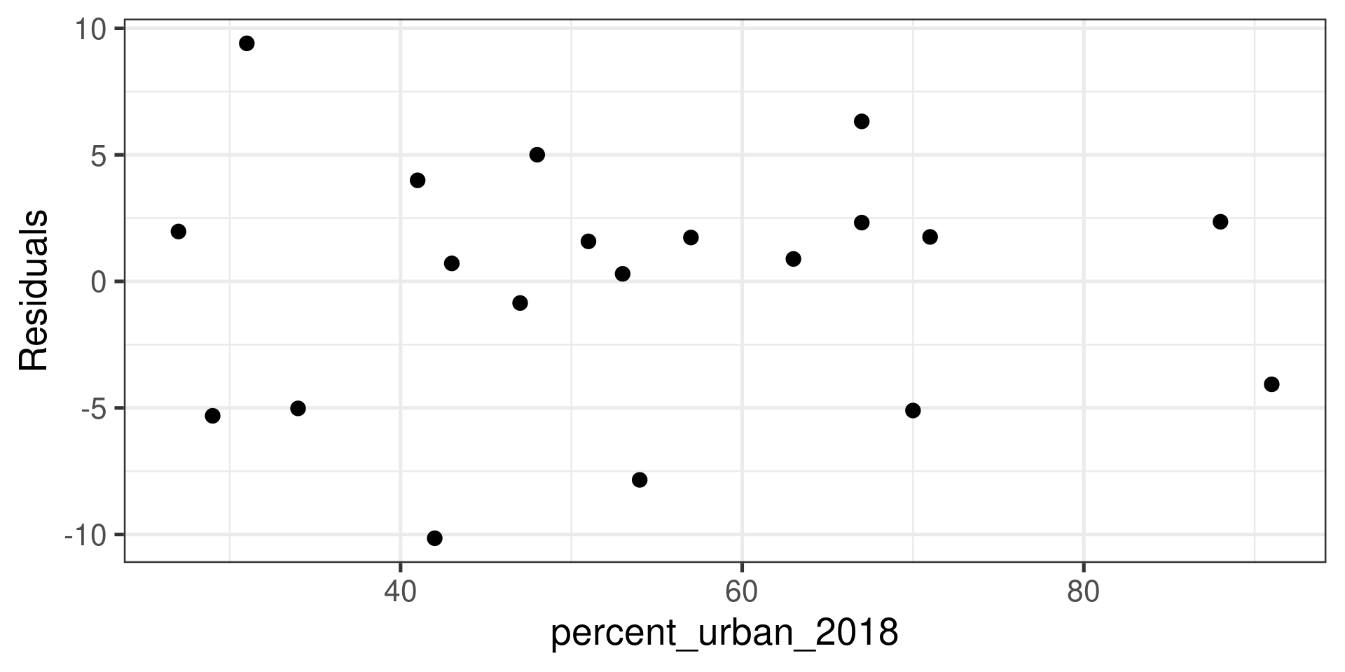
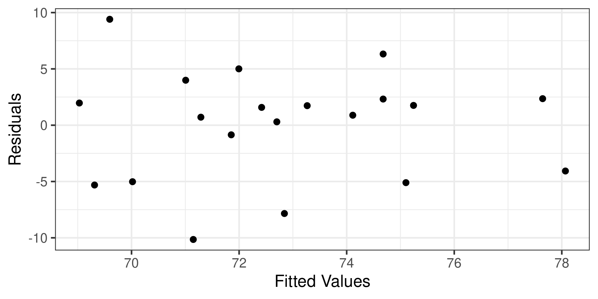
Residuals

model$residuals
          1           2           3           4           5           6 
  1.5812752   0.2988491  -0.8538727   1.9703877   6.3218668   9.4055357 
          7           8           9          10          11          12 
  0.7109794  -4.0672458   5.0049142   3.9934054   1.7570147   0.8867189 
         13          14          15          16          17          18 
  1.7339970  -5.1017723  -5.3120383  -7.8423639   2.3218668 -10.1478076 
         19          20 
  2.3563933  -5.0181034 


model$fitted.values
       1        2        3        4        5        6        7        8 
72.41872 72.70115 71.85387 69.02961 74.67813 69.59446 71.28902 78.06725 
       9       10       11       12       13       14       15       16 
71.99509 71.00659 75.24299 74.11328 73.26600 75.10177 69.31204 72.84236 
      17       18       19       20 
74.67813 71.14781 77.64361 70.01810 

Residuals

model$fitted.values + model$residuals
 1  2  3  4  5  6  7  8  9 10 11 12 13 14 15 16 17 18 19 20 
74 73 71 71 81 79 72 74 77 75 77 75 75 70 64 65 77 61 80 65 


sowc_sample$life_expectancy_2018
 [1] 74 73 71 71 81 79 72 74 77 75 77 75 75 70 64 65 77 61 80 65

Residual Plot

Why Does Life Expectancy Varies Between Countries?

Why Does Life Expectancy Varies Between Countries?

model <- lm(life_expectancy_2018 ~ percent_urban_2018, data = sowc_sample)

model

Call:
lm(formula = life_expectancy_2018 ~ percent_urban_2018, data = sowc_sample)

Coefficients:
       (Intercept)  percent_urban_2018  
           65.2169              0.1412  


\(\widehat{\text{life_expectancy_2018}} = 65.217 + 0.141 \times \text{percent_urban_2018}\)

Why Does Life Expectancy Varies Between Countries?

The complete equation:

\[\text{life_expectancy_2018} = {\color{#44ee44} 65.217 + 0.141 \times\text{percent_urban_2018}} {\color{#F9BA02} + e}\]

  • Association with urbanization (the model)

  • Other variables unrelated to urbanization (the residuals)

Residuals

Why Does Life Expectancy Varies Between Countries?

  • Variation associated with urbanization (the model)

  • Variation associated with other variables unrelated to urbanization (the residuals)

Variation of Life Expectancy

\[\begin{gather} \text{Variation associated with urbanization}\\ +\\ \text{Variation unrelated to urbanization} \end{gather}\]

Question: What portion of the variation in life expectancy is the variation associated with urbanization?

What portion of the variation in live expectancy is explained by the model?

Measuring Variation with Variance

Question: What fraction of the total variance of life expectancy is explained by the model?

\[\frac{\text{Variance of predicted values}}{\text{Variance of life_expectancy_2018}}\]

Coefficient of Determination \(R^2\)

\[1 - \frac{\text{Variance of residuals}}{\text{Variance of life_expectancy_2018}}\]

Summary of the Model

summary(model)

Call:
lm(formula = life_expectancy_2018 ~ percent_urban_2018, data = sowc_sample)

Residuals:
    Min      1Q  Median      3Q     Max 
-10.148  -4.305   1.234   2.330   9.405 

Coefficients:
                   Estimate Std. Error t value Pr(>|t|)    
(Intercept)        65.21686    3.58200   18.21 4.84e-13 ***
percent_urban_2018  0.14121    0.06333    2.23   0.0387 *  
---
Signif. codes:  0 '***' 0.001 '**' 0.01 '*' 0.05 '.' 0.1 ' ' 1

Residual standard error: 5.03 on 18 degrees of freedom
Multiple R-squared:  0.2164,    Adjusted R-squared:  0.1729 
F-statistic: 4.972 on 1 and 18 DF,  p-value: 0.03873

Comparison of Models

glimpse(sowc_sample)
Rows: 20
Columns: 5
$ percent_urban_2018         <int> 51, 53, 47, 27, 67, 31, 43, 91, 48, 41, 71,…
$ pop_urban_growth_rate_2018 <dbl> 2.8, 0.2, 1.8, 2.2, 1.1, -0.2, 2.0, 4.5, 0.…
$ total_pop_2018             <int> 17248, 1390, 106651, 9101, 1189, 287, 98424…
$ life_expectancy_2000       <int> 68, 69, 69, 62, 78, 77, 69, 72, 74, 71, 72,…
$ life_expectancy_2018       <int> 74, 73, 71, 71, 81, 79, 72, 74, 77, 75, 77,…

Different Models

for life_expectancy_2018:

  1. Predicting from percent_urban_2018:

    model1 = lm(life_expectancy_2018 ~ percent_urban_2018, data = sowc_sample)
  2. Predicting from pop_urban_growth_rate_2018:

    model2 = lm(life_expectancy_2018 ~ pop_urban_growth_rate_2018, data = sowc_sample)
  3. Predicting from total_pop_2018:

    model3 = lm(life_expectancy_2018 ~ total_pop_2018, data = sowc_sample)
  4. Predicting from life_expectancy_2000:

    model4 = lm(life_expectancy_2018 ~ life_expectancy_2000, data = sowc_sample)

Model 1

summary(model1)

Call:
lm(formula = life_expectancy_2018 ~ percent_urban_2018, data = sowc_sample)

Residuals:
    Min      1Q  Median      3Q     Max 
-10.148  -4.305   1.234   2.330   9.405 

Coefficients:
                   Estimate Std. Error t value Pr(>|t|)    
(Intercept)        65.21686    3.58200   18.21 4.84e-13 ***
percent_urban_2018  0.14121    0.06333    2.23   0.0387 *  
---
Signif. codes:  0 '***' 0.001 '**' 0.01 '*' 0.05 '.' 0.1 ' ' 1

Residual standard error: 5.03 on 18 degrees of freedom
Multiple R-squared:  0.2164,    Adjusted R-squared:  0.1729 
F-statistic: 4.972 on 1 and 18 DF,  p-value: 0.03873

Model 2

summary(model2)

Call:
lm(formula = life_expectancy_2018 ~ pop_urban_growth_rate_2018, 
    data = sowc_sample)

Residuals:
    Min      1Q  Median      3Q     Max 
-7.6117 -1.9358 -0.7584  2.1588  6.6903 

Coefficients:
                           Estimate Std. Error t value Pr(>|t|)    
(Intercept)                 77.0751     1.4092  54.695  < 2e-16 ***
pop_urban_growth_rate_2018  -2.1701     0.5406  -4.015 0.000813 ***
---
Signif. codes:  0 '***' 0.001 '**' 0.01 '*' 0.05 '.' 0.1 ' ' 1

Residual standard error: 4.127 on 18 degrees of freedom
Multiple R-squared:  0.4724,    Adjusted R-squared:  0.4431 
F-statistic: 16.12 on 1 and 18 DF,  p-value: 0.000813

Model 3

summary(model3)

Call:
lm(formula = life_expectancy_2018 ~ total_pop_2018, data = sowc_sample)

Residuals:
    Min      1Q  Median      3Q     Max 
-12.246  -2.135   1.464   3.509   7.505 

Coefficients:
                 Estimate Std. Error t value Pr(>|t|)    
(Intercept)     7.354e+01  1.480e+00  49.701   <2e-16 ***
total_pop_2018 -3.712e-05  4.039e-05  -0.919     0.37    
---
Signif. codes:  0 '***' 0.001 '**' 0.01 '*' 0.05 '.' 0.1 ' ' 1

Residual standard error: 5.554 on 18 degrees of freedom
Multiple R-squared:  0.04481,   Adjusted R-squared:  -0.008251 
F-statistic: 0.8445 on 1 and 18 DF,  p-value: 0.3703

Model 4

summary(model4)

Call:
lm(formula = life_expectancy_2018 ~ life_expectancy_2000, data = sowc_sample)

Residuals:
    Min      1Q  Median      3Q     Max 
-3.3240 -1.3480  0.2308  1.3781  4.2515 

Coefficients:
                     Estimate Std. Error t value Pr(>|t|)    
(Intercept)          25.11782    4.17523   6.016 1.09e-05 ***
life_expectancy_2000  0.69864    0.06083  11.484 1.02e-09 ***
---
Signif. codes:  0 '***' 0.001 '**' 0.01 '*' 0.05 '.' 0.1 ' ' 1

Residual standard error: 1.969 on 18 degrees of freedom
Multiple R-squared:  0.8799,    Adjusted R-squared:  0.8732 
F-statistic: 131.9 on 1 and 18 DF,  p-value: 1.02e-09

Multiple Regression

model5 = lm(
  life_expectancy_2018 ~ percent_urban_2018 + pop_urban_growth_rate_2018,
  data = sowc_sample)
summary(model5)

Call:
lm(formula = life_expectancy_2018 ~ percent_urban_2018 + pop_urban_growth_rate_2018, 
    data = sowc_sample)

Residuals:
    Min      1Q  Median      3Q     Max 
-6.0532 -2.0916  0.4063  1.9666  4.8125 

Coefficients:
                           Estimate Std. Error t value Pr(>|t|)    
(Intercept)                69.64133    2.52931  27.534 1.53e-15 ***
percent_urban_2018          0.13748    0.04182   3.288 0.004343 ** 
pop_urban_growth_rate_2018 -2.14419    0.43496  -4.930 0.000127 ***
---
Signif. codes:  0 '***' 0.001 '**' 0.01 '*' 0.05 '.' 0.1 ' ' 1

Residual standard error: 3.321 on 17 degrees of freedom
Multiple R-squared:  0.6775,    Adjusted R-squared:  0.6395 
F-statistic: 17.85 on 2 and 17 DF,  p-value: 6.649e-05