qt(0.975, df = 63)[1] 1.998341Summary of Inference Methods
Confidence level determines the accuracy of the method. This tells you how likely your interval is to “hit the target”.
Margin of error tells you how precise your estimate is. This tells you how precisely is the target determined when you hit it.
If you want to increase the accuracy, you have to decrease the precision, and vice versa.
You can increase one without sacrificing the other by increasing the sample size.
| \(H_0\) “true” | \(H_0\) “false” | |
|---|---|---|
| reject \(H_0\) | type I error | desired |
| don’t reject \(H_0\) | desired | type II error |
Researchers collected measurements of 64 zebra mussels (Dreissena polymorpha) from a lake in northern Michigan. The mean length of mussels in their sample was 37.5 mm, with standard deviation 7.2 mm. Use this data to find a 95% confidence interval estimating the mean length of the zebra mussels in the lake.
\(\overline{x} = 37.5\) mm
\(s = 7.2\) mm
\(n = 64\)
\(L = 0.95\) so \(\alpha = 0.05\)
Two-sided \(t^\star\):
qt(0.975, df = 63)[1] 1.998341\(\left(\overline{x} - m, \overline{x} + m\right) ={}\)
\(\left(37.5 - 1.7982, 37.5 + 1.7982\right) = {}\)
\(\left(35.7018, 39.2982\right)\).
We are \(95\)% confident that the interval \(\left(35.7018\text{ mm}, 39.2982\text{ mm}\right)\) contains the mean length of all the zebra mussels in the lake.
The length of zebra mussels in certain lake in northern Michigan was previously modeled using a normal distribution with mean 39.2 mm. In an attempt to control the zebra mussel infestation, native crayfish was introduced into the lake. Two years later, researchers collected measurements of 64 zebra mussels from the lake. The mean length of their sample was 31.8 mm, with standard deviation 6.1 mm. Use this data to test the original model at 5% significance level.
\(\displaystyle t = \frac{\overline{x} - \mu}{s/\sqrt{n}} = \frac{31.8 - 39.2}{6.1/8}\)
\({} = -9.704918\)
Two-tailed \(p\)-value with negative \(t\):
2 * pt(-9.7, df = 63)[1] 4.055363e-14We have sufficient evidence to reject \(H_0\) at 5% significance level.
Suppose an investigator takes a random sample of \(n = 50\) birth weights from several teaching hospitals located in an inner-city neighborhood. In her random sample, the sample mean \(\overline{x}\) is 3,150 grams and the standard deviation is 250 grams.
In a study on gifted children, the researchers collected data on the mother’s and father’s IQ of the 36 randomly sampled gifted children. The histogram below shows the distribution of mother’s IQ. Also provided are some sample statistics.
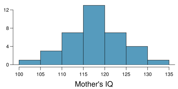
Perform a hypothesis test to evaluate if these data provide convincing evidence that the average IQ of mothers of gifted children is different from the average IQ for the population at large, which is 100. Use a significance level of 0.10.
A quality control engineer inspects 300 electronic components randomly selected from a large shipment. Exactly 18 of these components turn out to be faulty. Construct a 98% confidence interval giving the lower estimate of the proportion of faulty components in the shipment.
According to certain company regulations, a large shipment of electronic components must be returned to the manufacturer if more than 5% of the components are faulty.
A quality control engineer inspects 300 electronic components randomly selected from the shipment. Exactly 18 of these components turn out to be faulty.
At 2% significance level, is there sufficient evidence to support the decision to return the shipment?
What would a Type 1 error be?
What would a Type 2 error be?